Tutorial

A quick tour of what can be done with DeNSE.

A single neuron

First, one should import all the modules and variables that are necessary for the simulation:

import dense as ds
from dense.units import *

The first line makes the DeNSE simulator available and let us call it through the variable ds. The second line imports all the units (e.g. time units like ms, minutes…) which will be used to set the properties of the simulation and of the neurons.

Once this is done, we can create our first neuron:

n = ds.create_neurons()

This creates a default neuron without any neurites (a single soma). Let’s add an axon and a dendrite:

n.create_neurites(2, names=["axon", "dendrite_1"])

by default, neurons have their has_axon variable set to True, meaning that the first created neurite will be an axon and all subsequent neurites will be dendrites. Now that the neurites have been created, they can be accessed through n.axon and n.dendrites (or n.neurites to get all of them at the same time). We will set the parameters of the dendrite to make it grow more slowly than the axon. Because the default name of the first dendrite is "dendrite_1", this reads:

print("{!r}".format(n.axon))
print(n.dendrites)
print(n.neurites)

dprop = {
    "speed_growth_cone": 0.2*um/minute,
    "taper_rate": 0.01,
    "use_uniform_branching": True,
    "uniform_branching_rate": 0.05*cph
}

n.axon.set_properties({"speed_growth_cone": 0.5*um/minute})
n.dendrites["dendrite_1"].set_properties(dprop)

One can then plot and simulate the growth of this neuron:

''' Plot the initial state '''

ds.plot.plot_neurons()


''' Simulate a few days then plot the result '''

ds.simulate(7*day)
ds.plot.plot_neurons()

Two interacting neurons

Again, import all necessary modules and variables:

import dense as ds
from dense.units import *

Once this is done, we can set the various parameters for the simulation and the neuronal properties:

num_neurons = 2

simu_params = {

    "resolution": 1.*minute,
    "num_local_threads": num_omp,
    "seeds": [0, 1],
    "environment_required": False,
}

neuron_params = {
    "growth_cone_model": "simple-random-walk",
    "position": [(0., 0.), (100., 100.)]*um,
    "persistence_length": 200.*um,
    "speed_growth_cone": 0.03*um/minute,
    "taper_rate": 1./400.,
    "use_uniform_branching": True,
    "uniform_branching_rate": 0.009*cph,
}

neurite_params = {
    "axon": {"initial_diameter": 4.*um},
    "dendrites": {"taper_rate": 1./200., "initial_diameter": 3.*um}
}

The first line here declares the number of OpenMP processes that will be used, i.e. how many parallel threads will be used to perform the simulation. The second line will be used to set the number of neurons that will be simulated.

The third part contains the parameters related to the simulation: the timestep used to run the simulation, the number of threads used in the parallel simulation, the random seeds that will be used to generate random numbers (one per OpenMP thread), and whether the neurons are embedded in spatial boundaries.

Eventually, the neuron_params dictionary on line 11 contains the information that will be used to describe the growth of the two neurons, all expressed with their proper units (distances in microns, speed in micron per minutes, and branching events in ``counts per hour’’). As no environment was specified here, the positions of the neurons is also specified; there orientation (the direction of the axon) will be set randomly. Though we used the same parameters for both neurons here, this is not necessary and different parameters can be passed for each neurons through a list, as shown for the positions on line 15.

Once all these parameters are declared, we can configure DeNSE and create the neurons so that everything is ready for the simulation.

# configure DeNSE
ds.set_kernel_status(simu_params)

# create neurons
n = ds.create_neurons(n=num_neurons, params=neuron_params,
                      neurite_params=neurite_params, num_neurites=2)

As can be seen above, one uses the ds variable to access the simulator main function. The set_kernel_status() function is used here to transfer the parameters to the kernel of DeNSE (the main simulator units). Once this is done, the create_neurons() is called in order to obtain two neurons with the specific set of parameters declared in neuron_params, and two neurites (by default the first is an axon, and the second is a dendrite) which initially possess a single branch protruding from the soma.

Once the neurons are created one can visualize them using plot_neurons(). The initial condition of the neurons can thus be visualized before starting the simulation.

Following neuron creation, the simulation can be started and its result can be visualized again:

''' Plot the initial state '''

ds.plot.plot_neurons()


''' Simulate a few days then plot the result '''

ds.simulate(7*day)
ds.plot.plot_neurons()

After this first 7 day simulation, the parameters of the neurons can be changed to account for changes in developmental mechanisms, so that these new parameters can be used to simulate the next part of these cells’ growth.

''' Change parameters and simulate again '''

# new dendritic and axonal parameters
axon_params = {
    "speed_growth_cone": 0.02*um/minute,
}

dend_params = {
    "use_uniform_branching": False,
    "speed_growth_cone": 0.01*um/minute,
}

neurite_params = {"axon": axon_params, "dendrites": dend_params}

# update the properties of the neurons
ds.set_object_properties(n, neurite_params=neurite_params)

# simulate and plot again
ds.simulate(7*day)
ds.plot.plot_neurons()

Here we changed separately the dendritic and axonal parameters using the set_object_properties() function on the two neurons which are stored in the n variable (the neurons stored in a Population object).

Once the simulation is over, the shapes of the neurons that were obtained can be saved in standard morphology formats such as SWC or MorphoML (NeuroML). Note that the neuroml python module is necessary to use save_to_neuroml().

# In the swc format
ds.io.save_to_swc("neurons.swc", n)

Multiprocessing and random number generation

DeNSE support parallel simulations at the C++ level using OpenMP shared memory thread parallelism. Currently, the number of threads must be set at the beginning of a script, before any objects are created because objects are then allocated to a given thread which will be responsible for it. The number of thread can be set through

ds.set_kernel_status({"num_local_threads": 4})

if you want your simulation to run on four threads. Parallelism is implemented at the neuronal level: all neurites of a given neuron are associated to the same thread. There is therefore no point in allcating a number of threads which would be higher than the total amount of neurons in the simulation.

Warning

For people using simulateously DeNSE and other parallel simulation software, make sure that you or the software used do not set the OMP_NUM_THREADS variable to a value other than that used for DeNSE: this would lead to undefined behavior.

Since DeNSE also uses random numbers to make most of the actions associated to growth cone navigation, you can seed the random number generators used during the simulation through:

ds.set_kernel_status({"seeds": [1, 5, 3, 6]})

Note that one seed must be given for each thread. The result of a simulation should always be the same provided the number of threads and seeds used are identical.

Interactions and simulation speed, various tips

Simulation speed with DeNSE will vary greatly depending on the time resolution and interactions. By default, DeNSE uses a 1 minute timestep, with neuron-neuron interactions turned on, which can lead to rather long simulation times. To increase speed, several approaches may or may not be attractive to you.

• Increasing the time resolution. Using ds.set_kernel_status({"resolution": 5.*minute}), you can reduce the number of steps necessary to complete the simulation; this also has another advantage because it increases the size of the compartments composing the neuron, thus reducing their number and speeding up the interactions. However, this will obviously make the final results more “crude”, as you subsample the real path of the neurites.

• Increase the value of the "growth_threshold_polygon" kernel parameter; this parameter is related to the distance the growth cone must move away from its previous position for a polygon to be generated, at which point other growth cones will be able to interact with this new part of the branch. This brings speedups that are similar to increasing time resolution for the same reason mentioned previously: fewer geometric operations and polygons to deal with. Note that increasing this value could lead to approximations: growth cones that should have interacted may miss one another if you increase this value too far (over a few microns, for instance), though it remains very low for values below a micron.

• Switch the interactions off using ds.set_kernel_status({"interactions": False}). Neuron-neuron interactions are currently the main source of CPU requirement and, though we know how we could reduce them further, it is a non-trivial task for which we currently do not have the necessary time. If you are interested an would like to help on that, feel free to contact us.

• Do not use a spatial environment. Though this leads to lower speed gains compared to the other solutions, it might also help in specific cases.

Embedding neurons in space

One of the original aims for DeNSE was the study of neuronal cultures and devices, where the neurons can be embedded in more or less complex structures. In the simulator, simple spatial structures such as disks or rectangles can be generated directly from the Shape object. For more complex shapes, pre-constructed images in SVG or DXF formats can be imported using the culture_from_file() function.

''' Configuring the simulator and the neuronal properties '''

num_omp = 5
num_neurons = 50

simu_params = {
    "resolution": 10.*minute,
    "num_local_threads": num_omp,
    "seeds": [i for i in range(num_omp)],
    "environment_required": True,
    "interactions": False,
}

# configure DeNSE
ds.set_kernel_status(simu_params)


''' Create and set the environment '''

env = ds.environment.Shape.rectangle(500*um, 500*um)

ds.set_environment(env)

Once the environment is created, we can seed randomly the neurons inside it.

soma_radius = 4.*um
pos = env.seed_neurons(num_neurons, soma_radius=soma_radius, unit="um",
                       return_quantity=False)

Warning

Setting the soma radius correctly is critical, otherwise the soma might “protrude” out of the environment, which will lead to issues for neurite creation.

We can then create the neurons:

neuron_params = {
    "growth_cone_model": "simple-random-walk",
    "position": [tuple(p) for p in pos]*um,
    "persistence_length": 200.*um,
    "speed_growth_cone": 0.03*um/minute,
    "soma_radius": soma_radius,
    "use_uniform_branching": True,
    "uniform_branching_rate": 0.009*cph,
}

axon_params = {
    "initial_diameter": 4.*um,
    "max_arbor_length": 1.*cm,
    "taper_rate": 1./400.,
    "initial_diameter": 4.*um,
}

dend_params = {
    "initial_diameter": 3.*um,
    "max_arbor_length": 500.*um,
    "taper_rate": 1./200.,
    "initial_diameter": 3.*um,
}

neurite_params = {"axon": axon_params, "dendrite": dend_params}

# create neurons
n = ds.create_neurons(n=num_neurons, params=neuron_params,
                      neurite_params=neurite_params,
                      num_neurites=2)

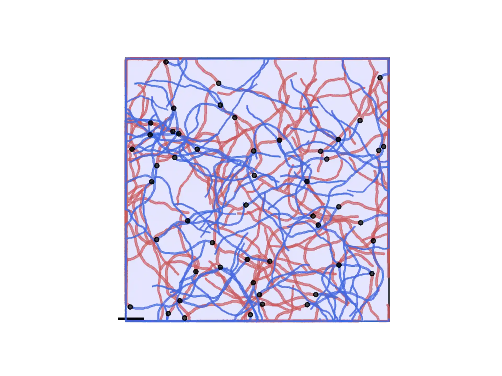
And simulate:

ds.simulate(4*day)
ds.plot.plot_neurons(scale_text=False)

Which leads to the following structure:

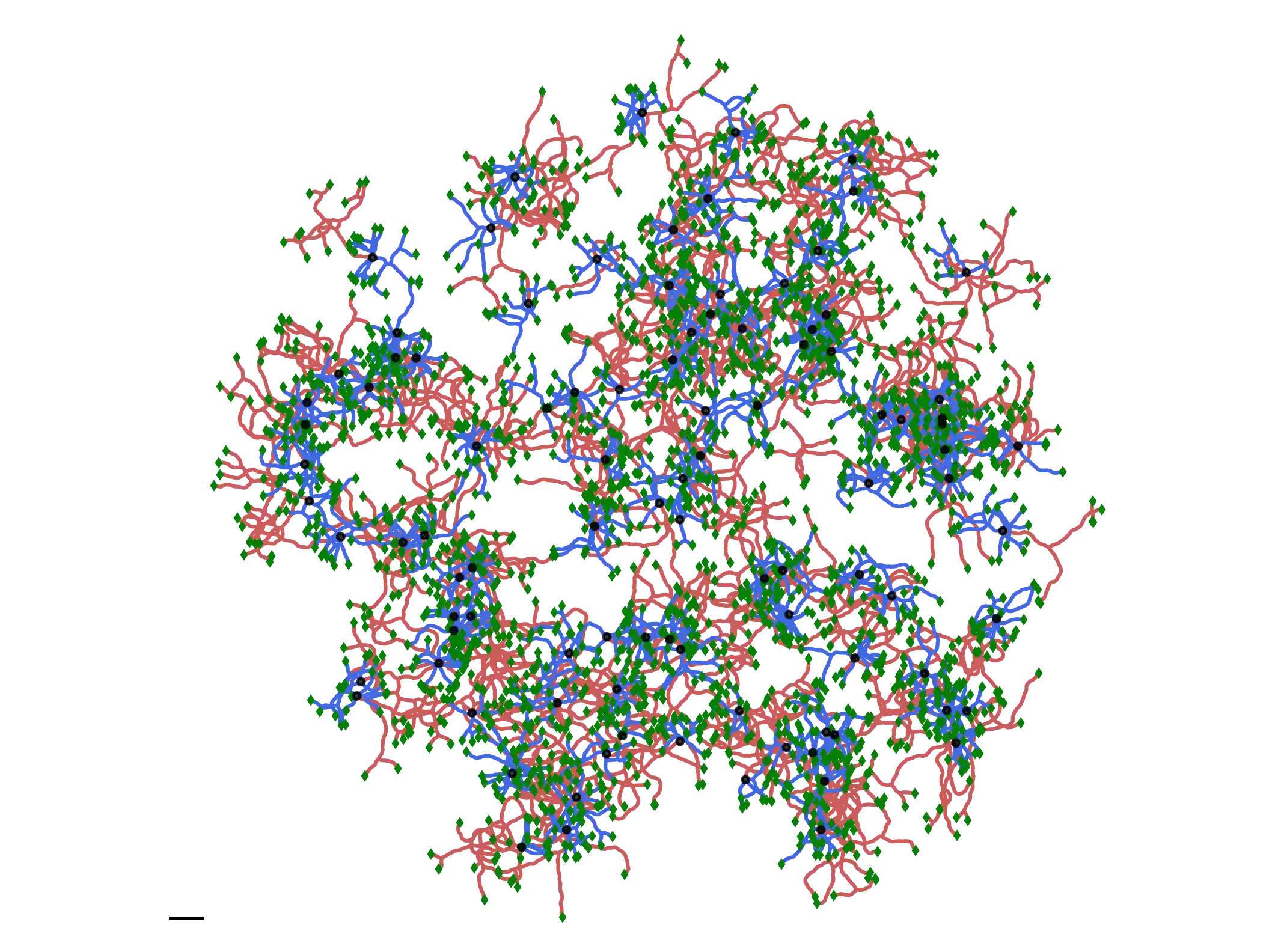
Complex neurons and parameters (Acimovic2011)

If you want to make a full neuronal network, you will probably want to specify specific neuronal shapes that can vary depending on the neurons. In this tutorial file, we show how to reproduce a study [Acimovic2011] using DeNSE.

This focuses especially on reproducing the shape of pyramidal neurons, with their specific neurite orientations and having varying number of neurites.

To do so, we start by defining the orientations for all possible neurites (between 4 and 6, with always at least an axon, an apical, and 2 basal dendrites) as well as their names.

'''
Neuronal parameters
'''

num_neurons = 100
num_pyr     = 80
num_nonpyr  = 20

density = 100 / (um**2)
radius = 564.2*um

soma_diam = 10.*um

neuron_params = {
    "growth_cone_model": "simple-random-walk",
    "soma_radius": 0.5*soma_diam,
    "use_van_pelt": True,
    "persistence_length": 100.*um,
    "random_rotation_angles": True,
}

# pyramidal parameters

neurite_angles = {
    "axon": 0.*deg,
    "apical": 180.*deg,
    "basal_1": 75.*deg,
    "basal_2": -75.*deg,
    "basal_4": 45.*deg,
    "basal_5": -45.*deg
}

names = list(neurite_angles)

The combination of "random_rotation_angles": True and the specific angles means that all neurites will be randomly rotated “as a block” for each neuron.

Then we generate a random number of neurites for each neuron and generate the associated names:

pyr_num_neur = rng.integers(4, 6, num_pyr, endpoint=True)

neurite_names = [names[:n] for n in pyr_num_neur]

Because simulating many neurons can take time, in this example we set the kernel parameters so that neuron-neuron interactions are ignored and the progress of the simulation is printed:

kernel_params = {
    "resolution": resolution,
    "num_local_threads": num_omp,
    "interactions": False,
    "print_progress": True
}

ds.set_kernel_status(kernel_params)

Finally we set the parameters and create the neurons:

pyr_params = neuron_params.copy()
pyr_params["neurite_angles"] = neurite_angles

pyr = ds.create_neurons(num_pyr, pyr_params, num_neurites=pyr_num_neur,
                        neurite_names=neurite_names,

If you run the whole file, you will get the following structure (scale bar is 50 \(\mu m\)):

Other Examples

The examples/ folder contains a collections of different applications cases illustrating DeNSE functions.

Models

examples/models/ contains examples concerning growth models.

examples/models/neurons/ contains a collections of DeNSE models built to generate various neuronal shapes : pyramidal cells, Purkinje cells, multipolar cells, chandelier cells, starbus amacrine, etc… The models were hand tuned for a qualitative resemblance with the corresponding cell types.

examples/models/neurons/ is an example code for importing and displaying a morphology file in neurom format.

examples/models/competition/ illustrates resource-based elongation models.

examples/models/branching/ shows codes to explore the branching models.

examples/models/random_walks/ Contains a code to run successively different simulations with different persistence lengths for a random walk base growth cone model.

Space Embedding

examples/space_embedding/ contains examples to make neurons grow in spatially bounded regions:

• polygons/ shows an example of multiple neurons growing in a space limited region containing obstacles. The connectivity network is generated at the end of the simulation.

• patterns/ illustrates growing of neurons in a complex geometry.

• ordered_neurons/ shows a code to generate neurons placed at precise locations and with controlled initial orientation of dendrites.

• droplets/ shows a code to generate a neuronal network in a complex geometry.

examples/multi_chambers/ is a special case of space embedding, where the culture is made of different chambers that communicate through channels of different shapes.

Growth Studies

examples/growth_studies/ contants different applications how to study network growth:

• turning_angles/, where neurons arrive on an obstacle with different inclination

• turning_walls_exp/, where neurons arrive in a chamber with different angles of the opening funnel

• recorders/ shows the usage of recorders

References

Acimovic2011

J. Aćimović, T. Mäki-Marttunen, R. Havela, H. Teppola, and M.-L. Linne (2011). Modeling of Neuronal Growth In Vitro: Comparison of Simulation Tools NETMORPH and CX3D. EURASIP Journal on Bioinformatics & Systems Biology, 616382.